Jenkins and Consistency
I apologize for the lack of posts lately. I've been busy with a lot of things. That doesn't mean I haven't done any sabermetric work lately. As a little teaser to what I've been working on, I'll post 2 graphs with no explanation. I'll only say that if you've read "Curveball", you'll know what I'm up to.
posted by rluzinski at 12:22 AM
![]()
![]()

9 Comments:
you'll have to at least tell me what a robojenks is before i understand this.
A player that gets 4 AB a game and bats .250 for the year isn't going to get exactly 1 hit a game no matter how consistent of a player he is. Random luck will group his hits up in, well, random ways.
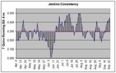
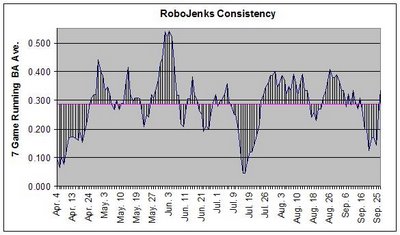
Jenkins batted .292 last year. That means that we can make a "Robot Jenkins" that always has a 29.2% chance of getting a hit during each AB and then run through a simulated season. The graph shows one example of the "inconsistency" a player like that would naturally show. Do that about 10,000 times and it represents the minimum or "expected" inconsistency a player will have.
By subtracting a player's actual consistency from their expected, you can begin to quantify how inconsistent a player is above and beyond the amount associated with dumb luck.
Wait a second, I said I wasn't going to explain this! ;)
Could you make another post some time in the future on what this is used for? Maybe explain the differences in the two graphs?
The look so different with the peaks and valleys in different places that I'm not sure what I'm supposed to notice.
Russ, you're expected consitency calcualtion is wrong. As you increase sample size you'll just approach the overall mean of the distribution, in this case .292. If you ran the simulations an infinte amout of time you'll end up with a horizontal line at .292. You need to look at the variance.
Russ, you're expected consitency calcualtion is wrong.
The graph wasn't meant to represent the average expected inconsistency; only an example of one season with an expected amount of inconsistency. Like you said, graphing the average inconsistency would be pretty darn boring, since it would just be a straight line right at Jenkin's BA last year.
To measure the expected inconsistency, I first find the average distance the running average is from the overall average for 1 season. I then run that 10,000 times and find that value's mean and standard deviation. I can then compare that to Jenkin's actual consistency numbers. It's very similar to the methodology used in "Curveball".
I planned on explaining all this on the next Brewerfan.net radio show, although I'm not sure if it's a subject matter that would work well in that format. I really shouldn't have posted the graphs here without explanation, however. I was only looking to generate a little interest. :)
My point was unless you do a measure across that distance (absolute value, squared diff) the mean should be zero.
I haven't explained this well. Each point on the graph is a 7 game rolling average. I then find the average distance that is from the overall batting average for a season. Well call this result "DIFF". In equation form:
DIFF = (ABS(rolling BA - BA))/(AB-6)
So, for one season, we might get a DIFF of .083 points. That means that after a 7 game average was established (after AB #7), the batter's rolling average was an average of 83 points from his overall BA.
Now, we can do the same thing with a simulation 10,000 finding the DIFF each time. The mean of that won't be zero, obviously. Knowing the simulated DIFF's mean and variance, we can compare that to the batter's DIFF and find the likelihood of the batter having his actual DIFF by chance alone.
That seems to be a bad measure if what you want to measure is "consistency." Now the big question is what you want consistency to mean. Under your current measure using .292 and .083 you treat a player hitting .335 one week and .250 the next the same as one hitting .292 one week and .209 the next. If you went to square difference you can then penalize large deviations from the mean.
That seems to be a bad measure if what you want to measure is "consistency."
Well, you'll have to take that up with the authors of "Curve Ball", since it's essentially their metric (I modified it slightly). I find it to be one valid way to quantify consistency, personally.
Under your current measure using .292 and .083 you treat a player hitting .335 one week and .250 the next the same as one hitting .292 one week and .209 the next.
I don't see how the 2 scenarios in the above example are obviously showing different extremes of consistency. That's not to say your proposed approach (squaring the diff.)is wrong (sounds perfectly valid to me) but neither is Curve Ball's, IMO. Just depends on...
Now the big question is what you want consistency to mean.
There's obviously no one definition and the above metric is only an example of one used by Curve Ball and myself to measure it. I also use longest hitting/hitless streak, most games with 3 or more hits, and games in a season spent with a DIFF of +/-.100 points (to capture extremes, like you proposed). I think those 5 metrics give a fairly comprehensive look at consistency.
I recommend you check out Curve Ball. It is one of the most repsected and recommended books in the sabermetric community. Not sure if this link will work, but it shows a scanned page of the book describing hitting streaks:
http://books.google.com/books?vid=ISBN038700193X&id=jqCujQ_Ww54C&pg=PA118&lpg=PA116&printsec=8&vq=hitting+streaks&dq=curve+ball&sig=xC_YEWCoaNT0bM-DEIvwbIBC0eE
Post a Comment
<< Home